Rule learning (differentiable ILP)

You can teach an xlog program two ways at once: write the rules you already know, and let the engine discover the rules you don’t. A loss you compute on a symbolic query flows all the way back into your PyTorch network’s weights, so logic and learning train together instead of in separate stages. Two features make this work, and they share one machinery:

A neural predicate turns a PyTorch network into a logical relation. Its facts carry probabilities that the network produces.
Differentiable ILP (Inductive Logic Programming — learning a rule from examples) searches candidate Datalog clauses with gradient descent and promotes the winner into your program.

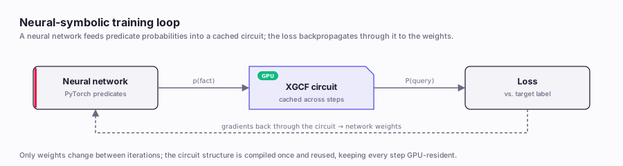
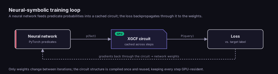
Both compile down to the same circuit and use the same gradient bridge. That is why a single loss can reach from a symbolic answer back to network weights.

Neural-symbolic training loop: a PyTorch network produces predicate probabilities, the cached XGCF circuit evaluates the query probability, a loss is computed against the target, and gradients flow back through the circuit to the network weights. — A loss on a symbolic query backpropagates through the cached circuit into the network's weights; only weights change between iterations.

When to use this

Reach for a neural predicate when you already know the rule but a fact’s truth depends on raw data — an image, an embedding, a sensor reading — and you want a network to supply that truth. Reach for differentiable ILP when you have examples of what should be true and want the engine to find the clause that explains them, rather than writing it by hand.

Neural predicates, differentiable ILP, and exact induction are distributed through the pyxlog PyPI wheel. This is a Python-first API; the crates published on crates.io do not expose it, so install pyxlog to use anything on this page.

Neural predicates

A neural predicate declares that a relation’s truth is decided by a network rather than by stated facts. You write the declaration in the program with ::, binding a registered network name to a predicate head:

nn(coin_net, [X], Y, [heads, tails]) :: coin(X, Y).

This is the four-argument form, nn/4. It reads: for input X, the network coin_net produces a distribution over the labels [heads, tails], and that distribution becomes the probability of coin(X, heads) and coin(X, tails). The label list makes this a classification predicate — the network output is a distribution over categorical labels. Drop the label list and you get the three-argument form, nn/3, an embedding predicate:

nn(embed_net, [X], E) :: node_embedding(X, E).

Here the network maps an input to a learned vector E instead of a label distribution. A given network may be declared in one form or the other, but not both. Declaring the same name as both classification and embedding is rejected at compile time.

Declarations are validated when the program compiles: input and output variables must be disjoint, every argument must appear in the bound predicate, and anonymous or aggregate variables are not allowed in a neural declaration.

Registering networks

The declaration only names a network. You supply the actual torch.nn.Module from Python at registration, which is where xlog wires the network into PyTorch’s automatic-differentiation (autograd) machinery so gradients can flow through it.

register_network(name, module, optimizer, scheduler=None, ...) binds a classifier, or nn/4 head. You pass the module and its optimizer, and optionally a learning-rate scheduler. The bridge holds them and drives the forward and backward passes through the circuit. Batching, top-k truncation, determinism, and a call cache are configurable here.
register_embedding(name, module_or_tensor, trainable=True) binds an nn/3 embedding — either a module or a plain tensor of vectors. Set trainable=False to freeze it.

Declaring the network’s shape

register_network takes three more keyword-only arguments that record what shape the network is: arity=, arg_sorts= and artifact_hash=. xlog does not take arity= on trust. It checks the number you pass against every nn/4 declaration bound to that name in your program, and a mismatch is a ValueError naming the predicate that disagreed. arg_sorts= needs one entry per declared argument, and passing it without arity= is refused — the sorts name the arguments, so there has to be an arity for them to name. program.network_metadata(name) reads the registration back together with the declarations it was checked against. For the coin classifier in the runnable example below:

program.register_network("coin_net", net, opt, arity=2)
program.network_metadata("coin_net")
# {'arity': 2, 'arg_sorts': None, 'artifact_hash': None,
#  'declared': [{'predicate': 'coin', 'predicate_arity': 2,
#                'input_arity': 1, 'labels': ['heads', 'tails']}]}

That is how you compare your own idea of a network’s shape against the program’s actual declarations, instead of trusting a naming convention. It raises ValueError if the name is not declared in the program, is declared as an embedding, or has not been registered yet. Once a network is registered, evaluating a query that touches the predicate does three things. It runs the network. It converts the output into probabilities on the circuit’s input nodes. And during training, it pushes gradients back through those nodes into the module’s parameters. The bridge also exposes forward_backward(query, expected=True), several differentiable losses (belnap_loss, semantic_loss_tensor, mse_loss_tensor), and epoch drivers (train_epoch, train_model) with optional validation-set early stopping.

Differentiable ILP

Writing a neural predicate assumes you already know the rule. Differentiable ILP is for the opposite case: you have examples of what should be true and want the engine to discover the clause. xlog frames this as learning which body to attach to a head. You mark a clause as learnable with a mask annotation:

learnable(mask) :: reach(X, Y) :- edge(X, Z), edge(Z, Y).

Compiling one candidate rule at a time is impossible at training timescales. So xlog instead pre-compiles a single tensorized graph — call it a super-graph — that holds every syntactically legal candidate body at once. A continuous mask tensor then decides which candidates are active. Each candidate gets a score (a logit). A Gumbel-Softmax relaxation — a differentiable way to make a soft, random pick among discrete options, controlled by a temperature τ — turns those scores into a soft selection over candidates. The circuit evaluates under that soft mask, a loss compares the derived facts against your examples, and the gradient updates the scores. As training proceeds, the temperature τ anneals toward a floor on a cosine schedule. Lower temperature sharpens the soft mask toward a single hard choice (one-hot). At convergence the engine takes argmax over the scores — it keeps the single highest-scoring candidate. That winner is decoded back into a concrete Datalog clause: a discrete rule string, not a soft mixture.

Sparse and dense mask backends

How the mask reaches the executor is chosen by a backend:

Backend	Parameters	When to use
`SparseMaskBackend` (default)	`O(C)` — one logit per candidate	Production. Ranks candidates on the device and pushes only the selected sparse set; no cubic tensor is materialized.
`DenseMaskBackend`	`O(N³)` — full schema cube	Debugging and parity checks. Enable with `debug_dense_mask=True`; it materializes the whole mask, so it is expensive on large schemas.

The sparse backend is what keeps training inside the GPU-resident hot loop: candidate probabilities are ranked and applied on the device, without downloading a full mask vector to the host CPU.

The Python training API

Two entry points drive learning, both in pyxlog.ilp. train_only(...) runs the search. It enumerates the legal candidates and launches several independent restarts from fresh scores. Each restart iterates the step loop: apply the mask, evaluate on the device, compute the loss, back-propagate, step the optimizer, anneal τ, and stop early once the argmax winner is stable and the loss is below threshold. It returns the discovered rule and its training telemetry. train_and_promote(...) wraps train_only with a set of promotion gates — checks a discovered rule must pass before xlog commits it into your program. A rule is written into your committed source only if it clears every gate:

Gate	What it checks
Convergence	Training actually reached a stable `argmax` winner.
Novel-rate	The rule does not over-derive facts outside the examples.
Protected-relation	It produces no unwanted side effects on protected relations.
Holdout F1	F1 on held-out examples meets the threshold (leave-one-out for small sets, k-fold for larger).
Ambiguity	No alternative candidate is a near-equal winner.
Typed-schema	Relation type metadata is present (or a reviewed waiver is supplied).

A rule that fails any gate is reported along with the gate it failed. It is never silently promoted.

Reliability gates

The search is stochastic, so different random seeds can converge or not. To keep that honest, dILP is held to seed-level reliability gates that grow stricter as the subsystem matures. A gate like 5/5 means “five consecutive runs must all succeed.”

Maturity	Gate	Meaning
Alpha	`5/5`	Five consecutive `train_only` runs must all converge.
Beta	`20/20`	5 seeds across each of 4 stages (reach, grandparent, colleague, plus-2) on the sparse backend — all 20 converge.
GA	`50/50`	50 seeds run against each of the 4 stages — 200 runs — scored with a Clopper–Pearson lower confidence bound on the success rate, a conservative statistical bound rather than a raw pass count.

A runnable neural-predicate example

This is a self-contained DeepProbLog-style program built on a single nn/4 declaration. A small classifier decides whether each coin image shows heads or tails, symbolic rules define winning and losing, and the network is trained purely from the derived symbolic queries. The synthetic tensors let it run without a dataset download.

nn(coin_net, [X], Y, [heads, tails]) :: coin(X, Y).

win(X, Y)  :- coin(X, heads), coin(Y, heads).
lose(X, Y) :- coin(X, tails).
lose(X, Y) :- coin(Y, tails).

import math
import torch
import torch.nn as nn
import pyxlog

DEVICE = "cuda" if torch.cuda.is_available() else "cpu"

# 2-class classifier over 3x64x64 coin images -> {heads, tails}
class CoinNet(nn.Module):
    def __init__(self):
        super().__init__()
        self.net = nn.Sequential(
            nn.Flatten(), nn.Linear(3 * 64 * 64, 64), nn.ReLU(), nn.Linear(64, 2)
        )
    def forward(self, x):
        return torch.log_softmax(self.net(x), dim=-1)  # log-probs over [heads, tails]

# Compile the program and bind the network to the nn(coin_net, ...) declaration.
program = pyxlog.Program.compile(open("coins.xlog").read())
net = CoinNet().to(DEVICE)
opt = torch.optim.Adam(net.parameters(), lr=1e-3)
program.register_network("coin_net", net, opt)

# Synthetic labelled coin images (even idx -> heads, odd idx -> tails).
labels = [i % 2 for i in range(16)]                    # 0=heads, 1=tails
images = torch.zeros(16, 3, 64, 64, device=DEVICE)
for i, y in enumerate(labels):
    images[i, y] = 1.0                                 # class-separable signal
program.add_tensor_source("train", images)

# Supervised atoms: coin(i, heads|tails). The label distribution is trained
# by back-propagating NLL through the circuit.
classes = ["heads", "tails"]
queries = [f"coin({i}, {classes[y]})" for i, y in enumerate(labels)]

for epoch in range(10):
    program.train_epoch(queries, batch_size=8)

# Inference: read a derived symbolic head's probability.
# nll_loss(q) is -log P(q), so exp(-nll_loss(q)) is P(q). It only evaluates —
# no gradient, no optimizer step.
def prob(query):
    return math.exp(-program.nll_loss(query))

print(prob("win(0, 2)"))   # both even -> both heads -> win fires high
print(prob("lose(1, 3)"))  # odd -> tails -> lose fires high

How you know it worked. After training, prob("win(0, 2)") is close to 1.0 — both inputs are even, so both classify as heads, so win fires. prob("lose(1, 3)") is close to 1.0 too, because odd inputs classify as tails. If both stay near their untrained values, the network did not learn the coin signal. nll_loss is the same quantity train_epoch minimizes, so you can also read it directly: a loss near 0 means the head is nearly certain, and a large loss means it is nearly impossible. Use evaluate_loss(queries) for the mean over a whole list. The optimizer here is Adam. On this multiplicative loss surface plain SGD tends to plateau, so Adam is the practical default.

Existential joins, mixtures, and graded masses

Existential-join trainable bodies (v0.10.0). A trainable body may join a neural predicate to an ordinary relation on a variable that is not in the head. The neural predicate is grounded over the real join domain inside the circuit, then combined at the head with a logical OR. Per-event features arrive through a domain_inputs= channel and register_domain_tensor_source. The join domain must be ground facts, and only a single join network is supported. Head-binding ids must be 0..N-1, row-aligned with your targets; the join domain’s own ids need not be dense — see domain_ids below. The planted graph is bounded (roughly six to seven events) by a fixed circuit buffer.
Joint multi-rule mixtures (v0.10.0). Several trainable clauses that share a head can be learned jointly as a noisy-OR mixture — a standard way to combine independent pieces of evidence into one probability. evaluate_joint_mixture reads the held-out result. A candidate may be guard-only, or it may carry a neural conjunct (neural_bodies=). That conjunct is a small trained head whose output is hard-thresholded (using a straight-through estimator, which passes gradients as if the threshold were smooth). The thresholded output acts as an on/off gate on the candidate’s eligibility, so it stays a derivation gate rather than soft truth mass.
Graded per-binding candidate masses (v0.10.0). train_neurosymbolic_program(..., candidate_masses={rule_id: tensor}) supplies per-binding confidences in [0, 1]. Each confidence multiplies into a candidate’s eligibility, so the head probability becomes the noisy-OR over graded evidence masses. Map head bindings to world steps and masses to a fact’s per-step confidence, and the guards train against an evolving trajectory. Omit the argument and the plain binary behavior is unchanged.
GPU-resident zero-host training step (v0.10.0). forward_backward_grouped(queries, expected) performs one host synchronization per step instead of a per-query round-trip, keeping the training loop resident on the device.
Row-addressed join domains (v0.11.0). train_neurosymbolic_program(..., domain_ids={net: [...]}) states which domain constant occupies each row of domain_inputs[net]. The ids may be given in any order but must be distinct, and the same list is handed to the engine and to the torch path, so both resolve a constant to its row the same way. Omit it and xlog assumes the dense identity 0..D-1, which it accepts only when the join relation’s domain is exactly that range.
Backbone coupling (v0.12.0). Set train_phi_gradient=True on a NeuralBodySpec and the entity features phi(x) are no longer detached on the training upload, so gradient reaches the feature producer too. It is off by default, and off is byte-identical to the previous path — only the autograd linkage changes, never the uploaded values.

The higher-level neuro-symbolic driver (pyxlog.ilp.neurosymbolic.train_neurosymbolic_program, with declarative trainable_rule(...) / train(...) in-source) is where the existential-join domain_inputs= channel is exposed.

Event-Calculus rule induction

Rules for when a situation starts and stops, learned from timestamped data — with the neural detector trained through the logic alone, and a statistical gate that abstains when the evidence is too thin.

Bounded exact induction

The non-gradient counterpart — deterministic GPU enumeration of candidate 2-body rules across four fixed topologies.

Python bindings

The full pyxlog API surface for registration, training, and querying.

Arrow and DLPack interop

How XLOG results and gradient tensors cross into PyTorch without a host round-trip.

Get Started

Core Concepts

Language Guide

Probabilistic Programming

Epistemic Reasoning

Neural-Symbolic

Guides

Rule learning (differentiable ILP)

When to use this

Neural predicates

Registering networks

Declaring the network’s shape

Differentiable ILP

Sparse and dense mask backends

The Python training API

Reliability gates

A runnable neural-predicate example

Existential joins, mixtures, and graded masses

See also

Event-Calculus rule induction

Bounded exact induction

Python bindings

Arrow and DLPack interop

​When to use this

​Neural predicates

​Registering networks

​Declaring the network’s shape

​Differentiable ILP

​Sparse and dense mask backends

​The Python training API

​Reliability gates

​A runnable neural-predicate example

​Existential joins, mixtures, and graded masses

​See also

Event-Calculus rule induction

Bounded exact induction

Python bindings

Arrow and DLPack interop

When to use this

Neural predicates

Registering networks

Declaring the network’s shape

Differentiable ILP

Sparse and dense mask backends

The Python training API

Reliability gates

A runnable neural-predicate example

Existential joins, mixtures, and graded masses

See also